#DIV/0! and #N/A really make me crazy! How can I make them go away?
Formula errors can be incredibly useful when you’re building spreadsheets because they help identify mistakes. However, there are many situations where errors are expected and displaying an ugly error message simply makes your worksheet look unprofessional.
Instead of showing #DIV/0!, #N/A, or other Excel error codes, you can replace them with cleaner values such as 0, a blank cell, or a custom message.
In this guide, we’ll look at the most common error-handling techniques in Excel and learn how to create cleaner, more user-friendly spreadsheets.
Understanding the #DIV/0! Error
The #DIV/0! error occurs when a formula attempts to divide a number by zero.
Imagine you’re calculating the ratio of widgets produced to widgets sold. The values in cells B3:E3 contain the number of widgets made, while B4:E4 contains the number of widgets sold.
- If no widgets were sold during a particular period, the value in the denominator becomes zero. Since division by zero is mathematically impossible, Excel displays a #DIV/0! error.
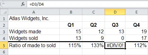
A #DIV/0! error occurs when a formula attempts to divide a number by zero.
- For many businesses, zero values are perfectly normal. Rather than displaying an error, it often makes more sense to show a zero or another meaningful result.
Using IF to Prevent #DIV/0! Errors
A common solution is to check whether the denominator contains zero before performing the division.
Traditional Approach
- =IF(D4=0,0,D3/D4)
This formula checks whether D4 equals zero. If it does, Excel returns 0; otherwise, it performs the division.
Shorter Approach
Because Excel treats zero as FALSE and any non-zero number as TRUE, you can simplify the formula:
- =IF(D4,D3/D4,0)
This formula reads as:
- If D4 contains a value other than zero, divide D3 by D4.
- Otherwise, return 0.
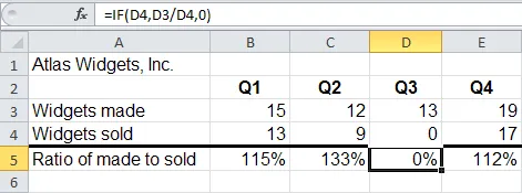
The first argument of the IF function usually contains a logical test such as D4=0, D4>0, or D4<>0. However, Excel automatically treats 0 as FALSE and any non-zero number as TRUE, which allows this useful shortcut.
Understanding the #N/A Error
Another common Excel error is #N/A.
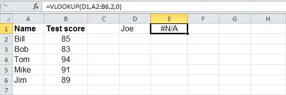
This error typically occurs when a lookup function such as VLOOKUP cannot find the requested value within the lookup range.
suppose you’re searching for the employee name joe within the range A2:A6.
- =VLOOKUP(D1,A2:B6,2,0)
If the value in D1 does not exist in the lookup table, Excel returns:
#N/A
While technically correct, displaying #N/A is often less helpful than showing a user-friendly message.
Replacing #N/A With a Friendly Message
Instead of displaying an error, you can return a custom message such as “Not Found”.
This approach allows users to immediately understand what happened without needing Excel knowledge.
For example, when a lookup value doesn’t exist in the lookup range, you might display:
Not Found
instead of:
#N/A
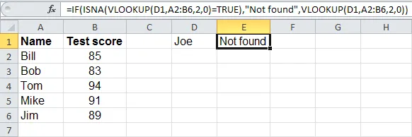
Bypassing the #N/A error.
Using ISERROR to Catch Errors
If you’re working in older versions of Excel, you can use the ISERROR function to detect errors before displaying a result.
- Handling Division Errors
=IF(ISERROR(D3/D4),0,D3/D4)
- Handling Lookup Errors
=IF(ISERROR(VLOOKUP(D1,A2:B6,2,0)),“Not Found”,VLOOKUP(D1,A2:B6,2,0))
The ISERROR function checks whether a formula returns any Excel error. If an error exists, Excel displays the alternative value you specify.
Using IFERROR (Recommended)
Starting with Excel 2007, Microsoft introduced the much simpler IFERROR function.
- Syntax =IFERROR(formula,value_if_error)
This function evaluates a formula and automatically returns a replacement value whenever an error occurs.
- Division Error
=IFERROR(D3/D4,0)
- Lookup Error
=IFERROR(VLOOKUP(D1,A2:B6,2,0),“Not Found”)
Compared to the ISERROR approach, IFERROR formulas are easier to read, easier to maintain, and often calculate faster.
Why IFERROR Is Better
Using IFERROR offers several advantages:
- Cleaner formulas
- Easier maintenance
- Better readability
- Faster calculations in many cases
- Handles most common Excel error types automatically
If you’re using Excel 2007 or later, IFERROR is generally the preferred solution for error handling.
Best Practices for Handling Formula Errors
To keep your spreadsheets clean and professional:
- Use IFERROR whenever possible.
- Check denominators before division.
- Replace lookup failures with meaningful messages.
- Display blanks instead of errors in reports and dashboards.
- Use error handling only when errors are expected during normal operation.
- Investigate unexpected errors rather than hiding them.
Final Thoughts
Errors such as #DIV/0! and #N/A are a normal part of working with Excel. While they are useful during development and troubleshooting, they can make finished reports look cluttered and confusing.
By using functions such as IF, ISERROR, and especially IFERROR, you can create cleaner spreadsheets that are easier for users to understand and more professional in appearance.
Frequently Asked Questions
Why does Excel display a #DIV/0! error?
The #DIV/0! error appears when a formula attempts to divide a number by zero or by a blank cell that Excel interprets as zero. Since division by zero is mathematically impossible, Excel returns this error.
How can I prevent a #DIV/0! error from appearing?
You can use the IF function to test whether the divisor is zero before performing the calculation.
- =IF(D4,D3/D4,0)
This formula returns the division result when D4 contains a non-zero value and returns 0 when D4 is zero.
Why does the formula =IF(D4,D3/D4,0) work?
Excel treats zero as FALSE and any non-zero number as TRUE. Therefore, if D4 contains a value other than zero, Excel performs the division. If D4 is zero, Excel returns 0.
What causes a #N/A error in Excel?
A #N/A error occurs when a lookup function such as VLOOKUP cannot find the requested value in the lookup range.
How can I replace a #N/A error with a custom message?
You can use IFERROR to return a custom value instead of displaying the error.
=IFERROR(VLOOKUP(D1,A2:B6,2,0),“Not Found”) What does the ISERROR function do?
ISERROR checks whether a formula returns any Excel error. If an error is detected, it returns TRUE; otherwise, it returns FALSE.
Can ISERROR handle more than just #DIV/0! and #N/A errors?
Yes. ISERROR can detect most common Excel errors, including:
- #DIV/0!
- #N/A
- #VALUE!
- #REF!
- #NAME?
- #NUM!
What is the IFERROR function?
IFERROR is an error-handling function available in Excel 2007 and later that evaluates a formula and returns an alternative value whenever an error occurs.
How is IFERROR different from using IF and ISERROR together?
IFERROR combines both operations into a single function.
Instead of:
=IF(ISERROR(D3/D4),0,D3/D4)
You can simply write:
=IFERROR(D3/D4,0)
When should I use IFERROR?
Use IFERROR whenever an error is expected as part of normal worksheet operation and you want to display a cleaner result such as:
0
A blank cell
“Not Found”
A custom message
instead of an Excel error code.